🐷 Susie Basic Timing and Ephemeris Object Usage#
🔵 Import the necessary python libraries and Susie objects.
import numpy as np
import pandas as pd
from susie.timing_data import TimingData
from susie.ephemeris import Ephemeris
import matplotlib.pyplot as plt
Matplotlib is building the font cache; this may take a moment.
🔵 Basic Usage#
The basic creation and usage of the TimingData and Ephemeris objects. This will assume the following:
Your data is in JD TDB timing format and system
You have both transit and occultation data
You have mid time uncertainties included in your data
We will pull this data from the repository below.
🔷 STEP 1: Download the timing data (that includes occultations) from the GitHub repository#
url = 'https://raw.githubusercontent.com/BoiseStatePlanetary/susie/refs/heads/main/example_data/wasp12b_tra_occ.csv'

# Read the CSV file directly from the URL
data = pd.read_csv(url)
tra_or_occs = np.array(data["tra_or_occ"])
epochs = np.array(data["epoch"].astype('int'))
mid_times = np.array(data["mid_time"])
mid_time_errs = np.array(data["mid_time_err"])
🔷 STEP 2: Add your transit and occultation data to the TimingData object.#
# Create new transit times object with above data
timing_obj1 = TimingData('jd', epochs, mid_times, mid_time_uncertainties=mid_time_errs, tra_or_occ=tra_or_occs, time_scale='tdb')
🔷 STEP 3: Create the Ephemeris object and add your TimingData object.#
ephemeris_obj1 = Ephemeris(timing_obj1)
🔷 STEP 4: Fit your transit time data to an ephemeris model. You can specify what type of model with the options ‘linear’ or ‘quadratic’.#
🔹 The Linear Model#
# Getting a linear model will solve for period and conjuction time (and their respective errors)
linear_model_data = ephemeris_obj1.fit_model('linear')
/home/docs/checkouts/readthedocs.org/user_builds/susie/envs/latest/lib/python3.12/site-packages/susie/ephemeris.py:100: RuntimeWarning: divide by zero encountered in divide
  period_tra = np.divide(mid_time_diff_tra, epochs_diff_tra)[-1] if x[tra_mask].size > 0 else np.nan
🟢 EXAMPLE#
Calling fit_model will return a dictionary of data. Below is an example of the dictionary returned for linear_model_data:
{'period': 1.0914196400440928,
 'period_err': 4.21033087274383e-08,
 'conjunction_time': 0.0023543850341696416,
 'conjunction_time_err': 9.256430832207615e-05,
 'model_type': 'linear',
 'model_data': array([2.35438503e-03, 2.53757421e+02, 2.58123099e+02...])}
# Uncomment this ↓↓↓↓ to see the real data!

# for key, value in linear_model_data.items():
#     print(f"{key}: {value}\n")
🔹 The Quadratic Model#
We can do the same process for a quadratic model by specifying ‘quadratic’ for the model type instead of linear. The same process above is shown below for the quadratic model.
# Getting a quadratic model will solve for period, conjuction time, and period change per epoch (and their respective errors)
quadratic_model_data = ephemeris_obj1.fit_model('quadratic')
/home/docs/checkouts/readthedocs.org/user_builds/susie/envs/latest/lib/python3.12/site-packages/susie/ephemeris.py:234: RuntimeWarning: divide by zero encountered in divide
  period_tra = np.divide(mid_time_diff_tra, epochs_diff_tra)[-1] if x[tra_mask].size > 0 else np.nan
🟢 EXAMPLE#
Below is an example of the dictionary returned for quadratic_model_data:
{'period': 1.0914217244026556,
'period_err': 1.543206321797526e-07,
'conjunction_time': 0.0005511865218625013,
'conjunction_time_err': 0.00014528672879359023,
'period_change_by_epoch': -9.902087992310958e-10,
'period_change_by_epoch_err': 7.206633676288036e-11,
'model_type': 'quadratic',
'model_data': array([5.51186522e-04, 2.53756075e+02, 2.58121761e+02, 3.20878495e+02...])}
# Uncomment this ↓↓↓↓ to see the real data!

# for key, value in quadratic_model_data.items():
#     print(f"{key}: {value}\n")
🔹 The Precession Model#
# Getting a quadratic model will solve for period, conjuction time, and period change per epoch (and their respective errors)
precession_model_data = ephemeris_obj1.fit_model('precession')
/home/docs/checkouts/readthedocs.org/user_builds/susie/envs/latest/lib/python3.12/site-packages/susie/ephemeris.py:369: RuntimeWarning: divide by zero encountered in divide
  period_tra = np.divide(mid_time_diff_tra, epochs_diff_tra)[-1] if x[tra_mask].size > 0 else np.nan
🟢 EXAMPLE#
Below is an example of the dictionary returned for precession_model_data:
{'period': 1.0914196985313172,
 'period_err': 1.32187600804159e-07,
 'conjunction_time': 2456305.45536,
 'conjunction_time_err': 0.00015706406134456078,
 'eccentricity': 0.0010000000000000009,
 'eccentricity_err': 0.0005602519531796543,
 'pericenter': 2.0,
 'pericenter_err': 0.4577749036402396,
 'pericenter_change_by_epoch': 0.001,
 'pericenter_change_by_epoch_err': 0.0003538492772010009,
 'model_type': 'precession',
 'model_data': array([2454515.52672922, 2454769.28250952, 2454773.64818754...])}
# Uncomment this ↓↓↓↓ to see the real data!

# for key, value in precession_model_data.items():
#     print(f"{key}: {value}\n")
🔷 STEP 5: Get BIC Values#
We can get the BIC value for a specific model fit using the model data dictionaries returned from the fit_model method.
linear_bic_value = ephemeris_obj1.calc_bic(linear_model_data)
quadratic_bic_value = ephemeris_obj1.calc_bic(quadratic_model_data)
precession_bic_value = ephemeris_obj1.calc_bic(precession_model_data)

print(f"Linear Model BIC: {linear_bic_value}\nQuadratic Model BIC: {quadratic_bic_value}\nPrecession Model BIC: {precession_bic_value}")
Linear Model BIC: 386.71897985393696
Quadratic Model BIC: 184.99006009832587
Precession Model BIC: 398.67927230204737
And we can also get a $\Delta$ BIC value using the method calc_delta_bic. We only need to specify which two models we would like to compare, with the second model BIC value being subtracted from the first model BIC value ($\Delta$ BIC = BIC ${model1}$ - BIC ${model2}$). The function will create the models, calculate the BIC values, and return the $\Delta$ BIC value for you!
Keep in mind, it ONLY returns the $\Delta$ BIC value and not the other data calculated.
lq_delta_bic_value = ephemeris_obj1.calc_delta_bic("linear", "quadratic")
lp_delta_bic_value = ephemeris_obj1.calc_delta_bic("linear", "precession")
qp_delta_bic_value = ephemeris_obj1.calc_delta_bic("quadratic", "precession")

print(f"Linear vs. Quadratic \u0394 BIC: {lq_delta_bic_value}\nLinear vs. Precession \u0394 BIC: {lp_delta_bic_value}\nQuadratic vs. Precession \u0394 BIC: {qp_delta_bic_value}")
Linear vs. Quadratic Δ BIC: 201.7289197556111
Linear vs. Precession Δ BIC: -11.960292448110408
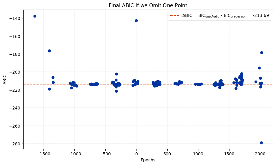
Quadratic vs. Precession Δ BIC: -213.6892122037215
🔷 STEP 6: Plot your data!#
Now you can use the model data dictionaries for plotting methods. Available plotting methods include:
plot_model: This will plot the model predicted mid-times. This takes in a model data dictionary.plot_timing_uncertainties: This will plot the range of uncertainties for the model predicted mid-times. This takes in a model data dictionary.plot_oc_plot: This will plot the observed mid-times minus the linear model predicted mid-times (calculated with $x=E$, $y=T_0-PE$, $y_{\rm err}=\sigma T_0$) and a curve(s) with the quadratic term ($x=E$, $y=0.5 \frac{dP}{dE} (E - {\rm median} (E))^2$) or the precession terms ($$). This DOES NOT take a model data dictionary.plot_running_delta_bic: This will plot how the $\Delta$ BIC value changes as observations increase over time. This DOES NOT take a model data dictionary.plot_running_analytical_delta_bic_quadratic: This will plot how both the numerical $\Delta$ BIC value and the analytical $\Delta$ BIC value changes as observations increase over time. This DOES NOT take a model data dictionary.plot_delta_bic_omit_one: This omits one data point at a time for each epoch and calculates the corresponding change in $\Delta$ BIC with that data point excluded.
🔹 Plot the model calculated mid-times#
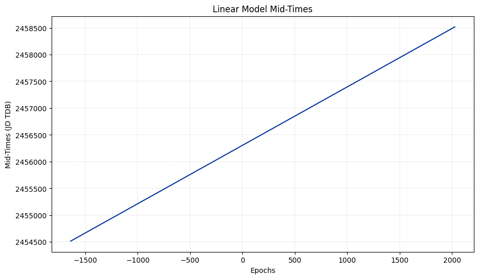
🔹 For the Linear Model
# Now we can plot this model
ephemeris_obj1.plot_model(linear_model_data, save_plot=False)
plt.show()
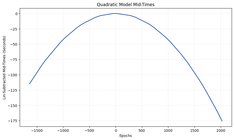
🔹 For the Quadratic Model
To see the quadratic effect in the data (which is very small compared to the linear term values) let’s use the subtract_lin_params argument in the method below with the value True. This will subtract the linear terms from the data so we can see the pattern of the smaller quadratic terms.
# Now we can plot this model
ephemeris_obj1.plot_model(quadratic_model_data, subtract_lin_params=True)
plt.show()
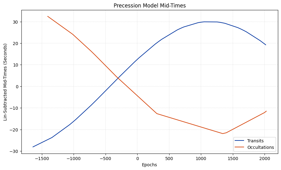
🔹 For the Precession Model
To see the non-linear effect in the data, we subtract the linear parameters as we did above by setting subtract_lin_params to True. We can also set the argument show_occultations to True to see the occultations plotted seperately.
ephemeris_obj1.plot_model(precession_model_data, subtract_lin_params=True, show_occultations=True)
plt.show()
🔹 Plot the model uncertainties#
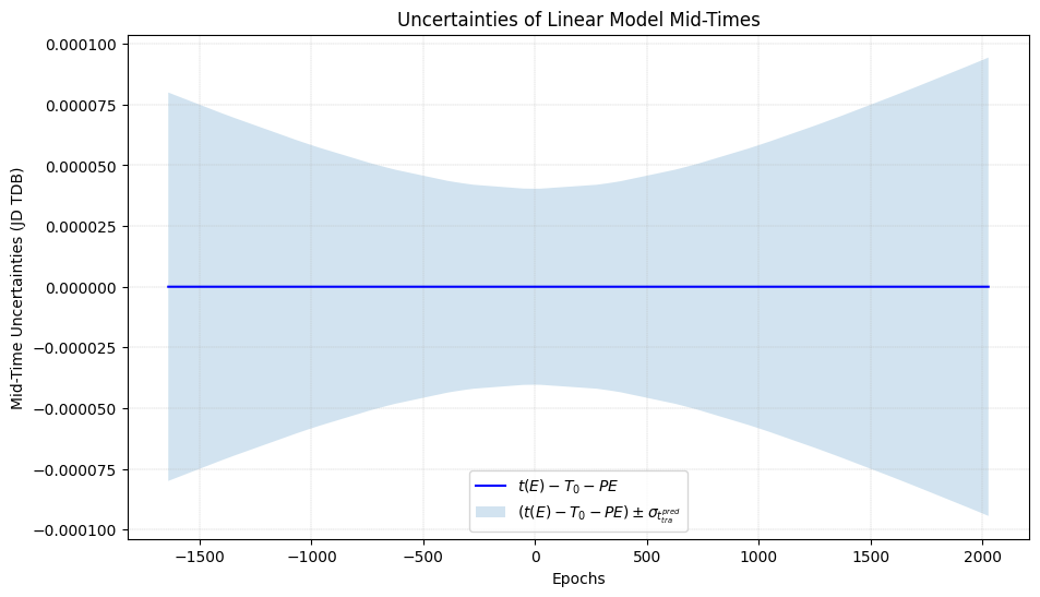
🔹 For the Linear Model
ephemeris_obj1.plot_timing_uncertainties(linear_model_data, save_plot=False)
plt.show()
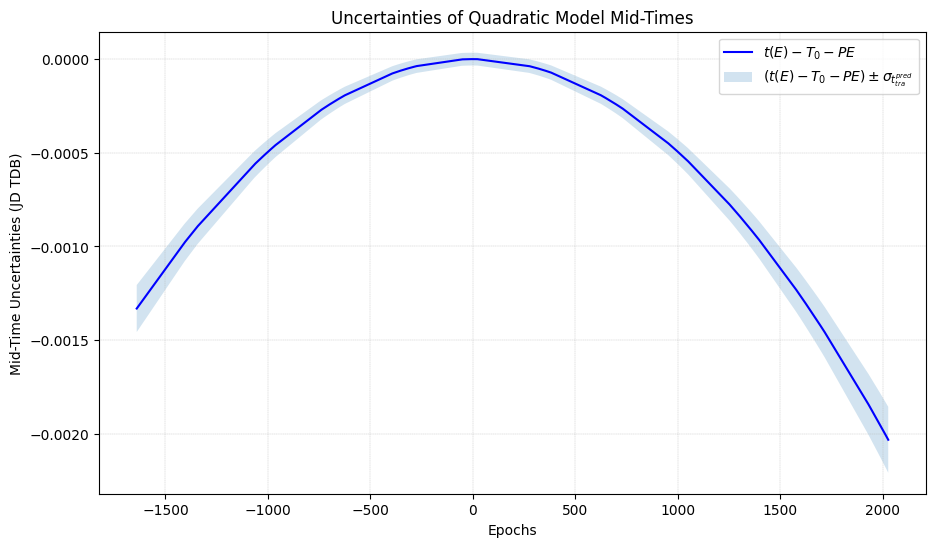
🔹 For the Quadratic Model
ephemeris_obj1.plot_timing_uncertainties(quadratic_model_data, save_plot=False)
plt.show()
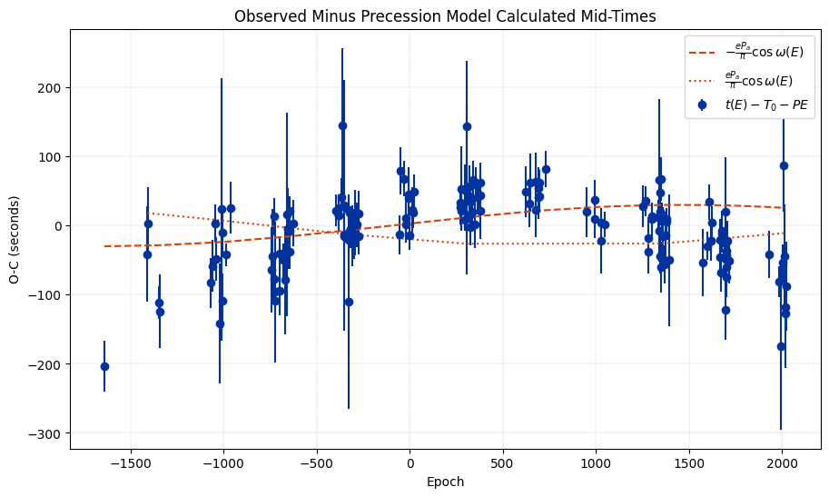
🔹 The O-C Plot#
ephemeris_obj1.plot_oc_plot("quadratic")
plt.show()

ephemeris_obj1.plot_oc_plot("precession")
plt.show()
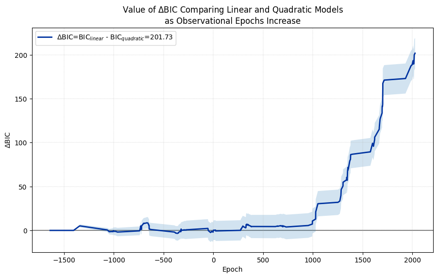
🔹 Plot the running $\Delta$ BIC#
Comparing a linear model and a quadratic model
ephemeris_obj1.plot_running_delta_bic("linear", "quadratic")
plt.show()
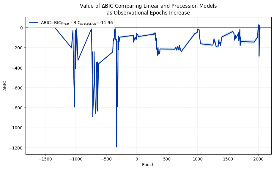
Comparing a linear model and a precession model
ephemeris_obj1.plot_running_delta_bic("linear", "precession")
plt.show()
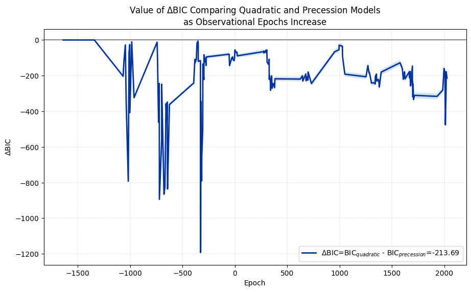
Comparing a quadratic model and a precession model
ephemeris_obj1.plot_running_delta_bic("quadratic", "precession")
plt.show()
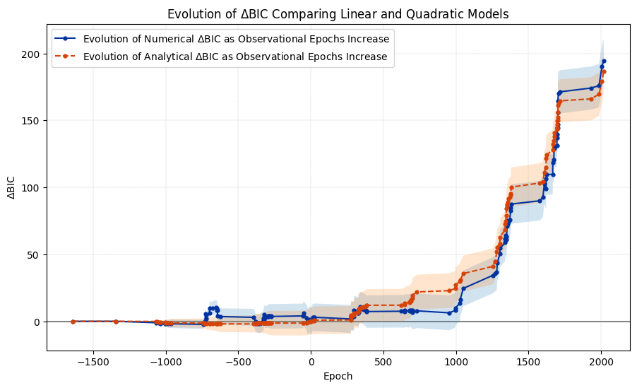
🔹 Plot the analytical running $\Delta$ BIC#
As of right now, this is only available for comparing a linear model and a quadratic model.
ephemeris_obj1.plot_running_analytical_delta_bic_quadratic()
plt.show()
/home/docs/checkouts/readthedocs.org/user_builds/susie/envs/latest/lib/python3.12/site-packages/susie/ephemeris.py:1918: RuntimeWarning: invalid value encountered in sqrt
  numerical_delta_bic_errs[i] = np.sqrt((2*(i-5)))
/home/docs/checkouts/readthedocs.org/user_builds/susie/envs/latest/lib/python3.12/site-packages/susie/ephemeris.py:1919: RuntimeWarning: invalid value encountered in sqrt
  analytical_delta_bic_errs[i] = np.sqrt((2*(i-5)))
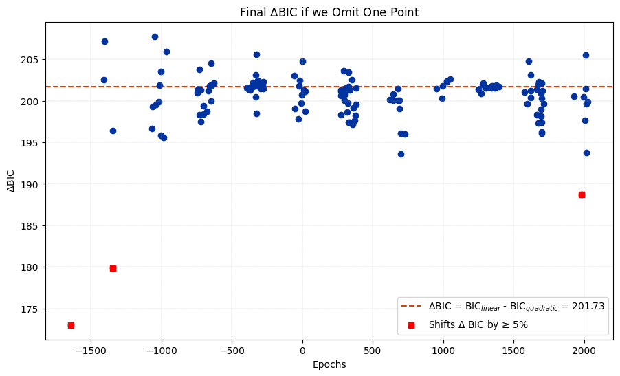
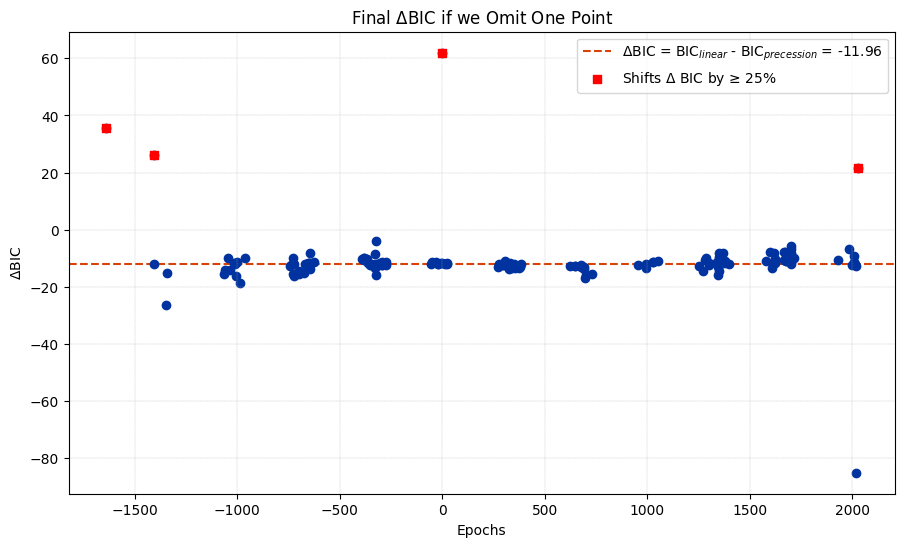
🔹 Plot the omit one $\Delta$ BIC#
For these plots, we have the option of highlighting outliers, or points that shift the value of $\Delta$ BIC by a specified percentage when omitted. We can specific the percentage we want to highlight using the argument outlier_percentage. For example, setting outlier_percentage to 25 will highlight any data point that shifts the value of $\Delta$ BIC by 25% or more.
Comparing a linear model and a quadratic model
ephemeris_obj1.plot_delta_bic_omit_one("linear", "quadratic", outlier_percentage=5)
plt.show()
Comparing a linear model and a precession model
ephemeris_obj1.plot_delta_bic_omit_one("linear", "precession", outlier_percentage=25)
plt.show()
Comparing a quadratic model and a precession model
ephemeris_obj1.plot_delta_bic_omit_one("quadratic", "precession")
plt.show()